Demystifying Deep Neural Networks
The beginner-friendly walkthrough of neurons, networks, and convolution I wish I'd had when I was starting out with Machine Learning.
Deep learning is a big topic and it can be pretty difficult to know where to start. When I first began learning about it, I found myself wading through very technical explanations with unfamiliar terminology and it was hard to abstract this away and develop an intuitive understanding of what is actually going on.
When I finally felt like I got my head round it I decided to create the explanation I wish I’d had access to. It’s aimed at people with some technical background and a basic grasp of maths (i.e. high-school level), but assumes no prior machine learning knowledge. There are a lot of simplifications, and a lot is missed out, but it’s my attempt to demystify neural nets and provide an ‘intuition’ that can serve as a foundation for further technical reading.
History
Despite their current buzz, neural networks are not a new concept. The idea of a biologically-inspired ‘perceptron’ was first explored in the 1940s, when the field was known as ‘cybernetics’. Unfortunately, some perceived limitations (such as the single-layer perceptron’s inability to model the XOR function) meant that it eventually fell out of favor.
In the 1980s, the field saw somewhat of a resurgence under the name ‘connectionism’. However, it was once again abandoned due to a lack of capable hardware and large datasets required for training to achieve good results.
‘Deep learning’ as it is currently known enjoyed yet another resurgence in the late 2000s. We now have more powerful computing hardware and GPUs optimized for training, as well as an abundance of freely available data on the internet. Could this mean that this time, neural networks are here to stay?!
Neural Nets vs Conventional Computing
Let’s try to understand how neural networks differ from conventional computing using a trivial example. If I wanted to write a conventional computer program to recognize images of cats, I would essentially have to chain up a whole load of ‘if’ statements:
`IF (furry) AND`
`IF (has tail) AND`
`IF (has 4 legs) AND`
`IF (has pointy ears) AND`
Etc…
Here, we are explicitly programming the computer for what features to look for. However, it’s pretty easy to see that these features could also apply to a dog or a fox, and it would be tricky to account for unusual edge cases like a cat without a tail or only three legs.
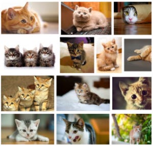
In a neural network on the other hand, we simply show the computer a load of examples of cats:
And a load of examples of not-cats:
Here, the computer works out what to look for, and what features are essential to ‘cat-ism’. This is actually a lot closer to the way humans learn to distinguish objects, and is why we call them ‘neural’ networks — they are inspired by biology and how our own brains work.
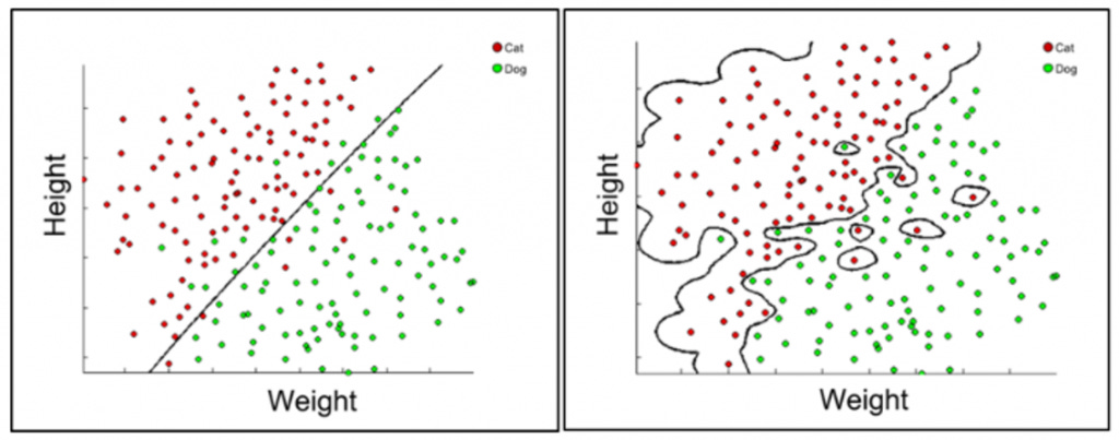
Here’s another way to think of it (this is actually a diagram illustrating a function created by a Support Vector Machine but I think the idea is still helpful in the context of neural networks):
On the left, a straight line attempts to separate the red dots (representing cats) from the green dots (representing dogs). While it does a relatively good job, there are still dots on the wrong side of the line. This would be a very easy function to model using conventional computing, using a straight line equation of the form:
y = mx + c
On the right, a much more complex function manages to successfully partition the dots, including weird outliers. It would be incredibly hard to write a function to describe this ‘line’ using conventional computing, but this is exactly the kind of complex function a neural network is able to learn, and it is clearly able to account for edge cases much better than explicit programming can. Here, we’ve only used two features (height and weight), whereas a neural network can handle many more features to learn a complex, robust, multidimensional model.
The best rule of thumb I have is:
Neural nets are good at things humans are good at (e.g. pattern matching), and bad at things computers are good at (e.g. maths and logic)
Inside a Neuron
Now let’s look at what happens inside a neuron. Again, we’ll use a trivial example to try and develop an intuition. Imagine I am trying to decide whether to go to a festival. I might consider things like:
Will the weather be nice?
What’s the music like?
Do I have anyone to go with?
Can I afford it?
Do I need to write my thesis?
Will I like the food?
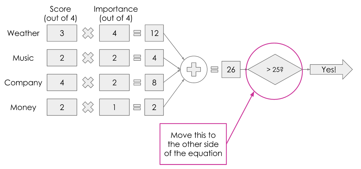
Let’s just take the first four for simplicity. To make my decision, I would consider how important each factor was to me, weigh them all up, and see if the result was over a certain threshold. If so, I will go to the festival! It’s a bit like the process we often use of weighing up pros and cons to make a decision. Let’s try and visualize this:
If I were to try and put some numbers on this, it might look something like this:
Let’s say the weather is looking pretty good but not perfect, so it gets a 3 out of 4. The music is ok but not my favorite, so it gets a 2 out of 4. Maybe my best friend has said she’ll come with me so I know the company will be great, so it gets full marks out of 4. Money-wise, maybe it’s a little pricey but not completely unreasonable so it gets a 2 out of 4.
Now for the importance: Maybe the weather is very important to me — I really want to go if it’s sunny, and I really don’t want to go if it’s not, so I give it a full 4 out of 4. Music-wise, let’s say I’m happy to dance to most things, so it’s not super important to me and I’ll give it a 2 out of 4. Similarly, I wouldn’t mind too much going to the festival on my own, so company can have a 2 out of 4 for importance. Finally, let’s say I’m feeling particularly flush at the moment so I’m not too worried about money, so I can give it just a 1 out of 4.
I multiply the value of each input by its weight, total this up, then check if it’s over a certain threshold — I’ve arbitrarily chosen 25 in this case. With these values, I get a total of 26, which is greater than 25, so I’m going to the festival!
For those of you who remember GCSE maths, you may recall that we can move operations to the other side of the equation:
Which would give us something like this:
This number is what is known as the ‘bias’ — it took me a while to get my head round where this mysterious ‘bias’ value came from when I started reading about neural nets!
Let’s take a look at this in its general form:
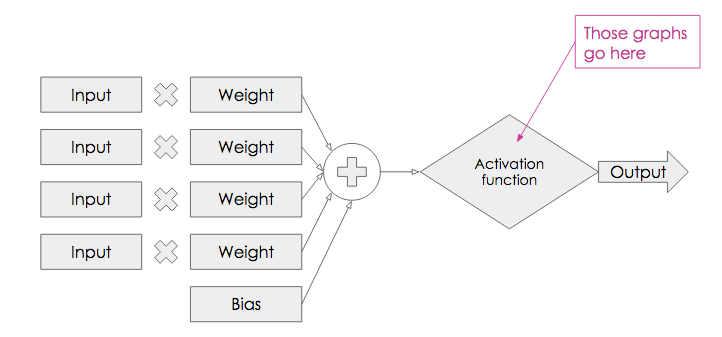
We have inputs that are each multiplied by a weight, summed up with a bias, put through what is known as an ‘activation function’ (in our case, the threshold test) and gives us an output.
Now, we have everything we need for a single neuron!
Constructing a Network
So how do we turn this from a single neuron into a neural network?
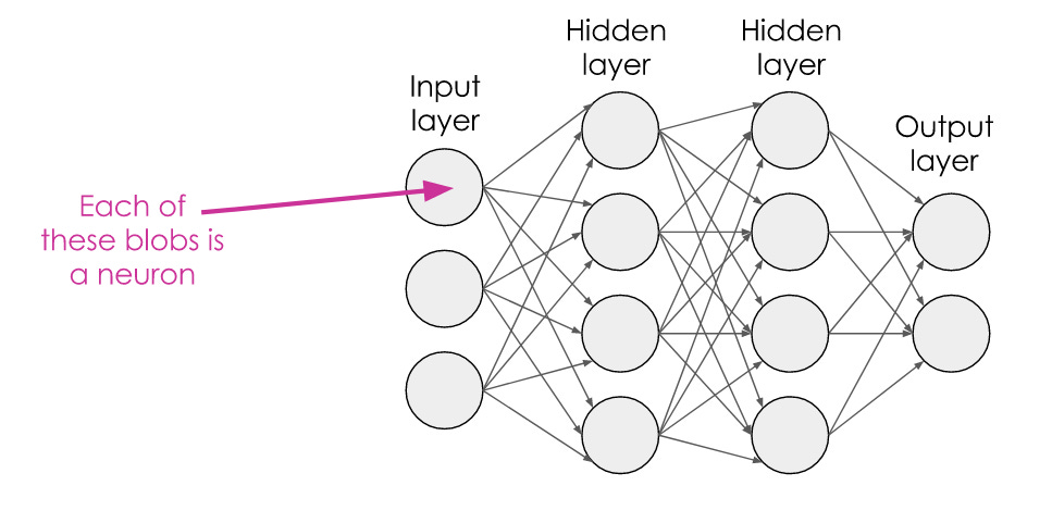
We simply chain up lots of them together! The outputs of the neurons in one layer flow through to become the inputs of the next layer, and so on.
And how do we turn this into a deep network? We simply add another hidden layer:
Generally, a neural network can be considered ‘deep’ if it contains more than one hidden layer.
Activation Functions
In our trivial festival example, we only had a binary output; yes or no — which we could achieve with a simple threshold test. But what if you want an output that isn’t binary? For this, we can use an activation function.
Here, we take the result of the sum part of the neuron and find it on the x-axis. We then read up along the y-axis to find the new output value. You can use any function you like, but there are a few that are commonly used:
The step function is what we have already seen: Below 0, our output is 0, above 0, our output is 1. The sigmoid function was popular historically as a kind of ‘smoothed out’ version of the step function which can give continuous values. It still gives a 0 at very low values and a 1 at very high values, but continuous values in between. The Rectified Linear Unit (ReLU) function outputs a 0 at values below 0, and outputs the input value at values above 0.
Just to return our model of a neuron, we can see where those graphs fit in:
So, we’ve done some multiplication, some addition, and some pretty straightforward reading off graphs.
Isn’t it all just simple arithmetic then?!
Unfortunately not. In our festival example, we hand-picked the weights and bias to give sensible results. This is easy to do for such a simple case. But for a problem involving many more features and a much larger multi-layered network, this is impossible. The computer itself needs to figure out what the values of the weights and biases should be. That’s the tricky bit! We do this by training the network.
Training the Network — the Short Version
Let’s look at an overview of the steps needed to train the network:
Randomly initialize the network weights and biases
Get a ton of labelled training data (e.g. pictures of cats labelled ‘cats’ and pictures of other stuff also correctly labelled)
For every piece of training data, feed it into the network
Check whether the network gets it right (given a picture labelled ‘cat’, is the result of the network also ‘cat’ or is it ‘dog’, or something else?)
If not, how wrong was it? Or, how right was it? (What probability or ‘confidence’ did it assign to its guess?)
Nudge the weights a little to increase the probability of the network more confidently getting the answer right
Repeat
Let’s visualize this.
Let’s assume we are training a network to differentiate between cats and dogs. We therefore only need two output neurons — one for each classification. We feed a cat image into the network. For now, imagine that each pixel of the image corresponds to one ‘input’ (we’ll see later how we can improve on this for images). Here, it’s assigned a probability of 62% that the image is a dog, and 38% that it’s a cat. Ideally, we want it to say this image is 100% cat.
So, we go backwards through the network, nudging the weights and biases to increase the chance that the network would classify this as a cat.
Training the Network — the Long Version
Now let’s take a deeper look at how we do this.
How do we know how wrong the network is? We measure the difference between the network’s output and the correct output using the ‘loss function’.
The loss function is also sometimes called the error function, energy function or cost function. Again, this took me a while to realize, so hopefully that will save you some time!
The best loss function will depend on your data and the intended application. We don’t have time to go into details about the different options, but in the spirit of encouraging intuition, a simple example of a loss function could be ‘mean squared error’ — this is what we learnt at school for fitting a line to data points — you try to minimize the squared distance between each of the points and the line:
A loss function is doing a similar thing, but in many, many more dimensions. They can get mathematically complicated, but it’s useful just to think of it as the difference between what the network does output and what it should output.
The goal of training is to find the weights and biases that minimize the loss function.
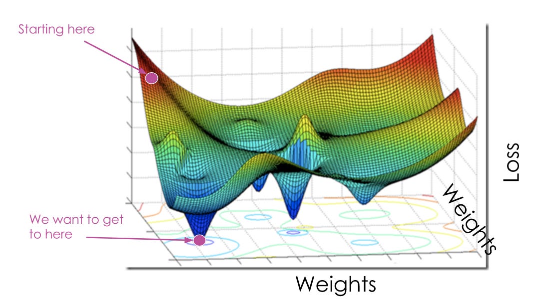
We can plot the loss against the weights. To do this accurately, we would need to be able to visualize tons of dimensions, to account for the many weights and biases in the network. Because I find it difficult to visualize more than three dimensions, let’s pretend we only need to find two weight values. We can then use the third dimension for the loss. Before training the network, the weights and biases are randomly initialized so the loss function is likely to be high as the network will get a lot of things wrong. Our aim is to find the lowest point of the loss function, and then see what weight values that corresponds to. It might look something like this:
Here, we can easily see where the lowest point is and could happily read off the corresponding weights values. Unfortunately, it’s not that easy in reality. The network doesn’t have a nice overview of the loss function, it can only know what its current loss is and its current weights and biases are. This is more like how the network sees it:
So how do we help the network find the lowest point?!
Gradient Descent
To find the lowest point, we use a technique called Gradient Descent. Imagine you are standing at the top of a mountain but have a blindfold on. You need to make it down to the bottom but you can’t see which way to go. What do you do? You feel around with your foot and find the direction that has the steepest slope, and then take a small step in that direction. You don’t want to take too big a step — that could be dangerous — but you also don’t want to take too small a step — it will take forever to get down.
So in terms of the network’s loss function, we find the direction of the steepest slope downwards, and take a ‘small step’ by nudging the weights a little in that direction.
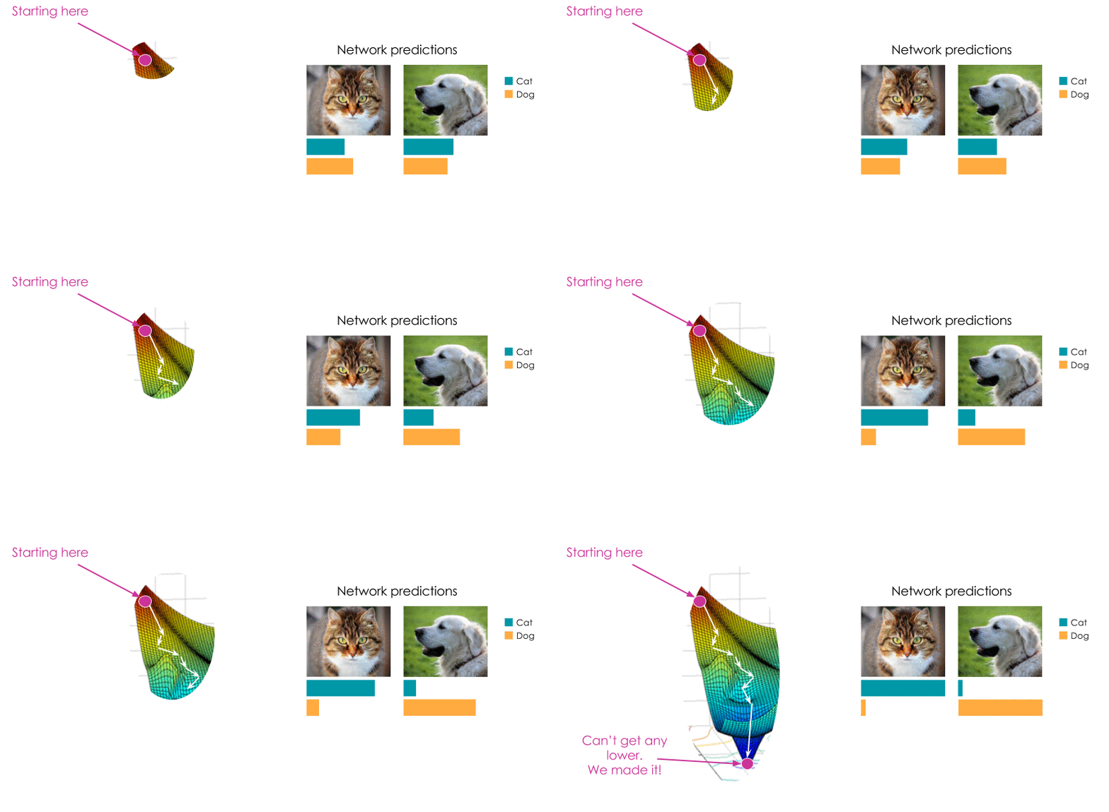
At first, the loss function will be high and the network will make incorrect predictions. As the weights are adjusted and the loss function decreases, the network will get better at outputting the right answers. Let’s try and visualize this:
As we descend the loss function ‘landscape’, the predictions of the network improve, as does its confidence.
Backpropagation
When reading about neural networks, you’ll often come across the term ‘backpropagation’. This refers to the algorithm used to perform gradient descent across the multiple layers of the network. The name comes from the fact that we start the process at the output layer, and work towards the input layer, propagating the changes backwards throughout the network. We calculate the gradient of the slope at each layer mathematically by taking the partial derivative of the loss with respect to the weights (if that makes no sense to you right now, don’t worry).
The amount we then nudge the weights in that direction is determined by the learning rate — this is the size of our ‘step’ down the mountain.
Don’t Panic!
That was quite a lot of technical detail given that I claimed this post was about creating intuition. But it’s ok, because there are loads of machine learning libraries that take care of the tricky maths. As long as you have a rough understanding of the overall process, you should know enough to read the documentation and start using these libraries. There are loads of options but one of the most popular at the moment is TensorFlow, Google’s open source machine learning library in Python. There are loads of great tutorials to help you get started.
Convolutional Neural Networks
Now let’s look at a special type of neural network called a ‘Convolutional Neural Network’, or ConvNet. Earlier, we visualized a cat image being fed into a neural network, and I said just assume each pixel corresponds to one input.
It turns out, there’s a more effective way to handle image data rather than assuming each pixel is independent.
If you think about an image, normally, pixels have a relationship with their neighbors (unless the image is of random noise). If I pick any random pixel of an image, it is quite likely that at least some of its neighbors are close to it in color. In other words, there is a kind of structure to the image where neighboring pixels tend to have some correlation.
ConvNets are specifically designed to take advantage of structure in input data. This is why they work so well for image processing and computer vision tasks.
Images Are Arrays of Numbers
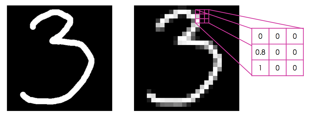
Here, I have pixellated an image of a hand-drawn number to illustrate this. In a monochrome image, each pixel has a value. In the example here, white pixels have a value of 1, black pixels have a value of 0, and grey is somewhere in between. The same principle is true of color images, but instead each pixel is defined by three numbers corresponding to the red, green and blue channels (sometimes there is a fourth number representing the ‘alpha’ channel which controls transparency).
Convolution
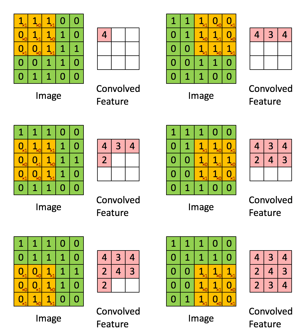
Because images are just arrays of numbers, we can do maths on them. A particularly useful mathematical operation we can do is called ‘convolution’. This involves passing another array of numbers over every pixel of the image, multiplying the overlapping numbers, adding them up, and creating a new array containing the results.
The array of numbers we pass over the image is called a ‘kernel filter’. Let’s say we have this kernel filter:
Let’s imagine convolving this with an image represented by the green array of numbers below. The red array represents the result of this convolution operation.
Convolving images in this way allows us to perform lots of ‘filter’ effects — many might seem familiar from image editing software like PhotoShop — this is exactly what happens when you apply a filter effect to your photos.
Depending on the values in the kernel filter, different results can be achieved.
Above, we see how different filters produce different effects. To blur an image, you essentially take an average of a pixel with its neighbors. To sharpen an image or detect edges, you amplify the pixel and de-weight its neighbors.
A Convolutional Neuron
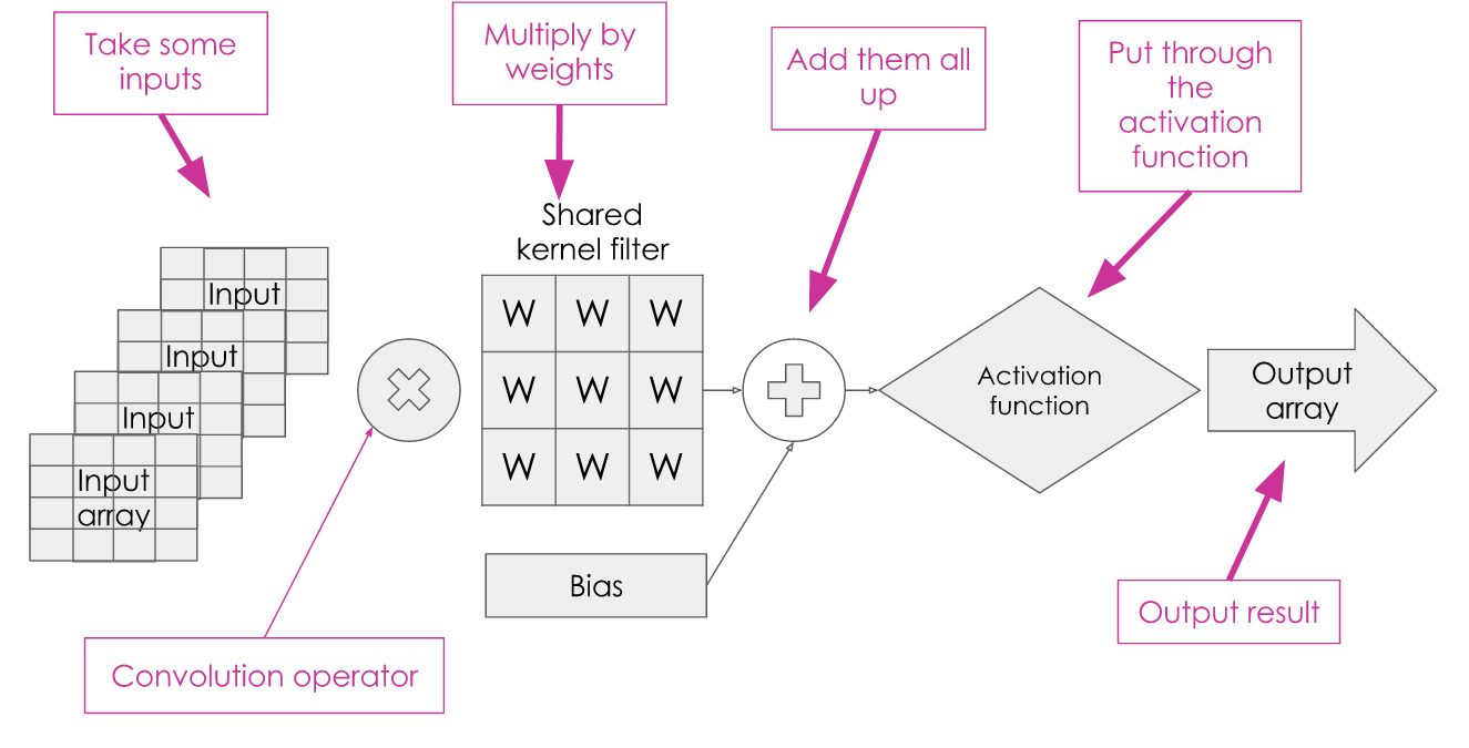
Remember our neuron from earlier? It looked something like this:
A convolutional neuron has got a very similar structure:
We have inputs; but instead of each being a single value we now take an array of values. Instead of multiplying the inputs by their own weights, we use the convolution operation with a shared kernel filter. The values within the kernel filter are what we need to work out by training the network. We sum the result with the bias and pass it through an activation function to get our output. With a convolutional neuron, the output is often an array rather than a single value.
What’s so Great About ConvNets?
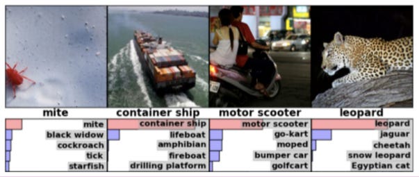
ConvNets have been making a splash in many image processing tasks. One example of this is the ‘ImageNet Challenge’, which asks teams to create algorithms to recognize objects given a labelled training data set.
Results of an algorithm in this challenge might look something like this:
As long as the correct object is within the algorithm’s top 5 guesses, it’s considered to have got it right. Until 2011, a good result in this challenge was around 25% error — so the algorithms would still guess incorrectly a quarter of the time, and a single percentage point was considered a good improvement.
When ConvNets were introduced in 2012, the error plummeted to just over 15% — an improvement of almost 10%! This was pretty extraordinary.
Teams continued to tweak ConvNets and in 2015, they actually outperformed humans at the task!
Inside a ConvNet
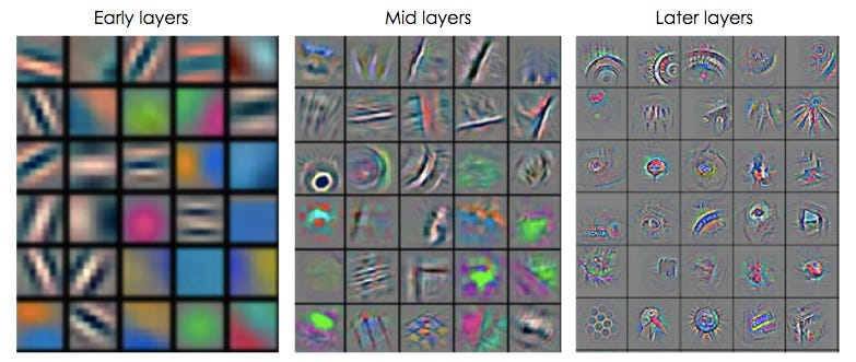
Remember we talked about how images are just arrays of numbers? And how kernel filters are also just arrays of numbers? This means we can actually visualize kernel filters as images. We can therefore see what weights have been learnt at different layers in the network, which helps us understand exactly how the ConvNet is learning to recognize objects.
Here, we can see that in the early layers, the network is learning very basic patterns: lines, edges and color patches — the fundamental building blocks of all objects. In the mid layers, the network has began to put these together into more recognizable structures: we can identify corners and curves. Finally, in the later layers, we start to see things that look much more recognizable as parts of objects, such as tires and boxes.
Apparently, this is not dissimilar to how our own human visual system perceives objects; another example of how neural networks imitate biology.
Fun Applications
A couple of years ago, Gatys et al noticed a very interesting consequence of ConvNets trained for object recognition. They realized that to identify an object, the network had to learn to abstract away the style of the image. The network should be able to recognize a cat whether it is a photo or a drawing, for example.
They found that the network was essentially siphoning off this stylistic information into certain layers of the network, so that it could be easily ignored. Similarly, certain layers were focused only on the content of the image, which were the layers primarily used for identifying the object.
This meant they could use the ‘style layers’ from one image and merge them with the ‘content layers’ of another image, resulting in an image taking on another image’s stylistic properties. They found they could the transfer the style of classic works of arts onto everyday photos:
In fact, this algorithm now powers an app called Prisma, which allows you to turn your selfies into masterpieces. I had a lot of fun experimenting with this…
Fooling ConvNets
Another fun (or worrying…) side effect of ConvNets is that they can be easily fooled.
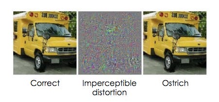
Here, an image of a truck was successfully identified by the network. Then, the researchers applied some distortion to the image that is imperceptible to the human eye — to us, it still looks very much like a truck. But to the ConvNet, this was now clearly an ostrich:
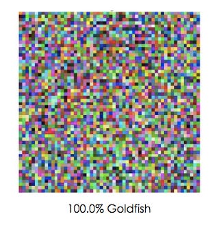
Similarly, the ConvNet confidently predicted that this image of random noise was in fact a goldfish:
Deep Dream
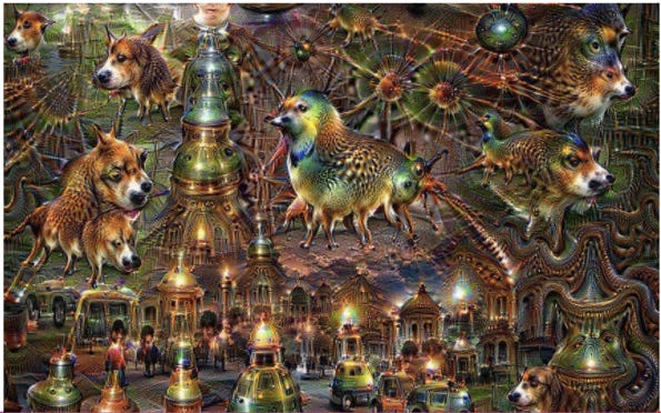
Google brought ConvNets into the limelight with their ‘Deep Dream’ experiments.
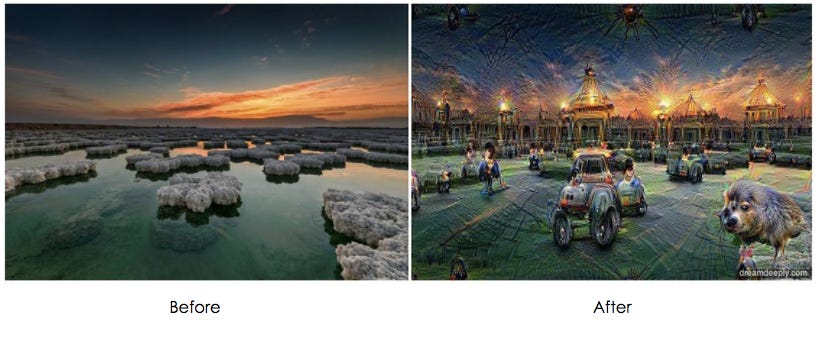
Here, they used a trained ConvNet but ran the process ‘in reverse’. Instead of nudging the weights, they nudged the image. This is effectively like telling the network ‘whatever you see in the image, enhance it!’
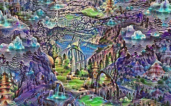
The results were these mysterious, dream-like hallucinations — earning the name ‘deep dream’ due to the idea that this could be what computers see when they dream.
Here are a few examples…
The network has dreamt up all kinds of shapes, with plenty of cars, building and dogs. Lots of dogs.
You might be wondering…
Why Are There so Many Dogs?!
The reason is that the ConvNet was trained on a dataset of images which included a lot of cars, buildings and dogs. This means it was predisposed to seeing these objects — kind of like human pareidolia: the bias that causes us to see faces in everything from clouds to toast.
This is actually a really interesting and important point. It can be tempting to assume that computers are objective and infallible, when in fact they are neither. We’ve seen a few examples of this. This is known as ‘algorithmic bias’, and as machine learning is used more and more it’s vital to be aware of this. The network only sees what it’s been trained to see.
This means that humans can accidentally (or sometimes intentionally) transfer their own biases and flaws, and networks can inadvertently learn proxies and correlations instead of real insight.
Phew! We Did It.
We’ve seen what’s in a neuron, how they make a network, what a ConvNet is and some of their interesting applications. But there is a ton we haven’t covered. When reading about neural networks, you might encounter words like: unsupervised learning, pooling, strides, stochastic, batch, dropout, regularization, transfer learning, recurrent neural networks, generative adversarial networks, and loads more. There is no way we can cover all this in one post! However, you should have a good foundation to go on and read about these things even more.
Also, Andrej Karpathy, one of the biggest names in ConvNets right now, tweeted this:
So in the words of an expert, a basic 4-layer ConvNet works best in real life.
And if you remember from earlier, we know about convolutional neurons, and we know about 4-layer networks, and we know we can use a library like TensorFlow to build them:
So you should have all you need to start building some useful stuff! Yay. Thanks for reading! Let me know if this has helped by leaving a comment or tweeting me @RosieCampbell

